
Splitting text in cells in Excel spreadsheets is a good skill to learn, especially if you are importing data. Often, imported data ends up all in one column, and it is tedious and a waste of time to manually re-type the data into new columns to be able to work with it all. Our step by step guide will help you save time and learn to effectively split data.
Download our splitting text in cells example and follow along.
Step 1:
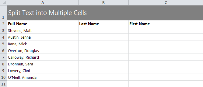
Choose the range of cells you want to be split. In the example this will be cells A3 through A10.
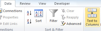
In the ribbon at the top, choose the “Data” tab and from there, select “Text to Columns”.
Step 2:
Once clicked, a dialog box will pop up. In this window, select “Delimited” and click next.
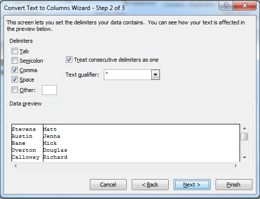
Once you are in the Delimiters section, you will have check boxes available. Select “Comma” and “Space” and leave the rest unchecked. Click next.
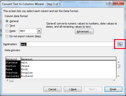
Step 3:
Click “Text” in “column data format”. After that, select the “option” button to the very right of the text box to indicate what columns you want to place the final output in.
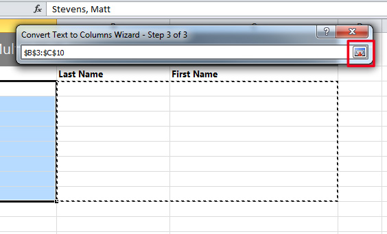
Now you will choose the range that you want Excel to put your output data. Once you have done this, press the far right button (indicated below) and wait for the final dialog box. Then click finish.
If you have followed the example guide, you’ll see that column B contains first names and column C contains last names. You can delete column A by right clicking “A” and selecting delete, moving the B & C columns over to the left.
Want to learn more about Excel? See our guides section.
Check this out while you wait!