Splitting Names in Excel

Learn the process for splitting names in Excel spreadsheets. When importing information into Excel, name data usually ends up all in one column, making it hard to alphabetize and organize. In this guide you will learn how to split the full name into three columns, one for the first name, one for the middle initial, and a third for the last name. Follow along to learn this Excel skill.

Download the example to practice these formulas.

Open the example spreadsheet and you can view all the full names in column A. The first step is to isolate the first names. Select cell B6 and enter the formula:

=TRIM(LEFT(A6,FIND(” “,LOWER(A6),1)))

Now B6 will contain “Jessica”.

Next is extracting the middle initial. Choose cell C6 and use this formula:

=MID(A6,FIND(” “,A6)+1,FIND(” “,A6,FIND(” “,A6)+1)-FIND(” “,A6)-1)

C6 will now show “M.”. The final part of this process is to isolate the last name so you can sort all parts of someone’s name however you want.

Go to cell D6 and enter the formula:

=TRIM(MID(A6,FIND(” “,LOWER(A6),FIND(” “,LOWER(A6),1)+1)+1,LEN(A6)-FIND(” “,LOWER(A6),1)+1))

D6 will show “Livingston” after you press enter. You have now officially split a full name into three organized sections.

Once you have completed this, you can apply this formula to all of the names without having to enter the formula over and over. Drag the cell that has already been filled (B6, C6, etc) down the column and it will fill in everyone’s name correctly. The formula is made to automatically adjust for each cell.

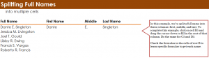
When you are using these formulas in your own Excel sheet, you need to change the instances of “A6” to the cell number of the full name you are referencing. For instance, the formulas for Dante E. Singleton contains “A5” instead of “A6”. This is how Excel knows where to pull information from.

See more Excel guides here.