
Learn the left formula in Excel. The left function for Excel takes characters from another cell starting with the left side character. This function can be used to abbreviate or simplify large amounts of data within your Excel spreadsheets. With our example guide, you will take the left characters from a name and put it into a new cell.
To begin, download the example spreadsheet.
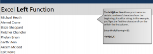
Open the example and you can see the A column is already populated with names. The B column is where you will take the names from the A column and place their partial info. The goal is to shorten each name to just the first 5 characters entered.
Select cell B3 and type:
=left(A3,5)
A3 is referencing what cell you want to retrieve data from, and the 5 is the indicating number of characters you want. You will get the result of “Micha”.
When using this formula on multiple names or entries, you don’t have to enter the formula in each cell. Instead, grab the corner of cell B3 and drag it to B10. This will fill in each of the B cells with the 5 left characters from the name next to them in column A. You can then click on any of the filled cells and change the formula if needed, or leave it as is.
To learn more Excel formulas, see our tutorials.
Check this out while you wait!