Highlighting Cells with Certain Values

In Excel, users are able to facilitate conditional formatting to highlight certain cells based on their contents.  This can be achieved with multiple “if statements”, however Excel makes it easier with conditional formatting as a function. Highlighting cells with certain values is done this way.

Download the example to learn how.

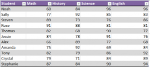
The example is of a spreadsheet with a grade book, and the goal is to highlight all of the cells that reach the value of 90% and above.

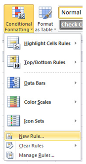
To begin, select the range of cells with the values you need. In the Ribbon’s Home tab, choose “Conditional Formatting” and then click “New Rule”.

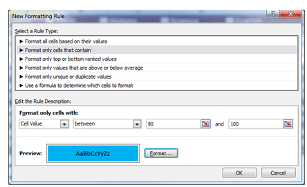
A dialog box will appear with options and from that select “Format only cells that contain”.

Proceed to the boxes near the bottom of the dialog and you will see the option “Format only cells with” and four drop down menus. Click the following options:

“Cell value”, “between”, “90 and 100”.

In the formatting button, select a text color and press OK.

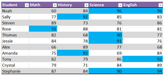
Your spreadsheet will now automatically display cells with the value of 90 and above with a different color background based on what you have previously chosen.