
In Excel, you have the ability to add drop down menus to any cell, row, or column. With these menus, you are able to access multiple data choices for output within a cell. To learn how to create drop down lists, read through the tutorial and make a drop down for employee departments.
Download the example spreadsheet to follow along.
Creating a Drop Down Menu in Excel
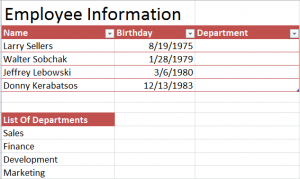
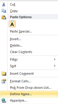
Click the “List of Departments” option in the example spreadsheet and drag the selection to highlight cells A9 through A13. Right click and choose “Define Name” from the list that comes up.
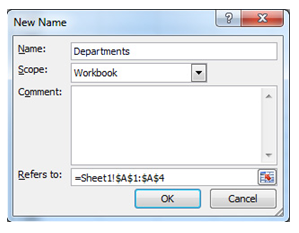
A dialog box titled “New Name” will open next. Enter a title for the list. We chose “Departments”.
Now your departments menu is created, you just need to tell Excel where to insert the list.
Highlight cells C3 through C6 together.
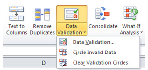
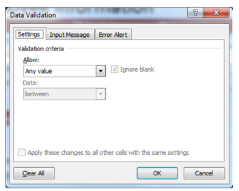
Go to the “Data” tab in the Excel Ribbon bar and click “Data Validation”, then pick the “Data Validation” option.
In the box that appears, make sure you’re on the first tab, the“Settings” tab. In the menu under “Allow”, click “List” and more options will be available. Click on the text box under “Source”:
Input the list name “=Departments” (without quotations) or the name you made earlier for the list (if it differs).
You can also customize messages for the drop down menu. This is done in the two tabs in the dialog box called “Input Message” and “Error Alert”.
When you have finished customizing your menu, press enter.
Under “Employee Information”, go to the empty “Department” cell next to an employee name and click on it to select it. A white drop down arrow can now be clicked, and the menu will display the options for each department. Choose from the list and the department name will be inserted.
Check this out while you wait!