
Creating a pivot table in Excel allows the user to quickly and easily summarize and arrange large amounts of data, and then pull certain details to view them.
Download the How to Create Pivot Tables in Excel tutorial to follow along.
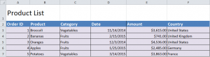
Start by choosing a cell inside the pre-filled data area from the example spreadsheet.
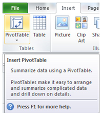
Click on the “Insert” tab at the top of the spreadsheet and choose “PivotTable” from the options.
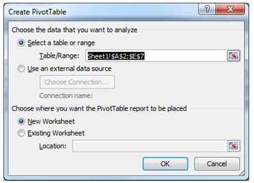
The “Create PivotTable” dialog box will come up after you’ve chosen this. It will indicate the range of the pivot table that can be created.
Choose if you want the Pivot Table to be in a new spreadsheet, or the example sheet you’re currently working on. Press OK after you’ve chosen.
The field list will appear on the screen. For this particular example, choose to add the following:
“Product Field to Row Labels”
“Amount to Values area”
“Country to Report Filters”
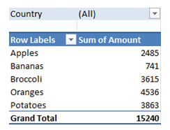
Through these, your Pivot Table has been made! It will look like this:
Check this out while you wait!