Using VLOOKUP in Excel

Excel’s VLOOKUP function allows a user to search through the first column in a certain cell range and return the data from a cell in the same row of that range. Using VLOOKUP in Excel is good for finding specific data quickly.

Download the example to use this function in the tutorial.

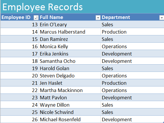
In the example spreadsheet, the VLOOKUP function is used to retrieve the full name or a department just by using the data of an employee ID in the formula.

The Syntax for VLOOKUP

VLOOKUP(lookup_value, table_array, col_index_num, [range_lookup])

This formula is put together through these indications:

Lookup_value – this is the value to search for.

Table_array – For the range of cells that contain the data desired.

Col_index_num – Indicates the number of the column in table_array that you want a matching value retrieved from.

Range_lookup – Optional for VLOOKUP, it determines if an exact match or an approximate result can be returned.

VLOOKUP in the Example

For this, you want to discover the full name of employee number 22 in your employee database using only the employee ID number.

Start with selecting cell A18 which is where you will begin building the VLOOKUP function.

Since we know the value (employee number 22) to search for already, in the first column enter:

=VLOOKUP(22,

Following this, enter in the range of the data you want searched through.

=VLOOKUP(22,a3:c16,

Choose the number of the column that has the data you are looking for, in this case “Full name” is column 2.

=VLOOKUP(22,a3:c16,2,

Since you wan an exact match on the result, close the formula with:

=VLOOKUP(22,a3:c16,2, FALSE)

Enter the full formula into cell A18. The result should be Martha Mackinnon if everything was entered correctly.