
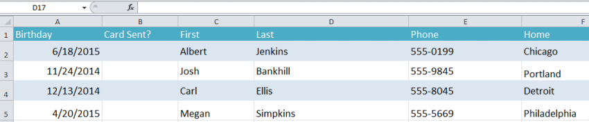

Applying conditional formatting to an Excel spreadsheet is great feature to know. The example in the tutorial shows how the Excel program can track birthdays of clients and note when a date has a passed. With conditional formatting, once a date has passed, the formula provided will mark the “Card Sent” cell with a “yes”.
Download the applying conditional formatting tutorial and follow along.
Begin with selecting cells A2 through A5.
Click “Conditional Formatting” in the Excel Ribbon Tool at the top, then “New Rule” from the drop down list.
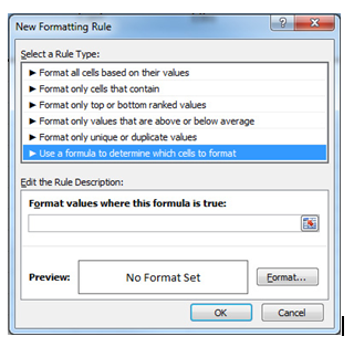
This triggers a dialog box. Click “Use a formula to determine which cells to format” to proceed.
In the example spreadsheet, input the format value text box with “=a2>TODAY()” and then click the “Format” option.
In the top “Font” tab, chose the color red and make the font bold. With these selected, the cell text will be bold and red if the birthday of the client is on a future date.
IF statements in Conditional Formatting
In the same example, select cell B2 and enter the following:
=IF(A2<TODAY(),”Y”,””)
This will read if the day indicated is in the past. If so, the formula will cause the cell to be marked with as “Y” for yes, which will tell you if you sent the client a card for their birthday.
Finally, drag the formula through cell B5 so all the cells in that column have the same formula applied. Use this conditional formatting technique for Excel documents that you want automatically updated.
Check this out while you wait!